Creating Word Clouds of Various Shapes
This post introduces how to create word clouds of various shapes using simple libraries and effective visualizations
Introduction
World clouds are the visual representation of text data of text data, typically used to depict keyword metadata on websites, or to visualize free form text. Google says a word cloud is “an image composed of words used in a particular text or subject, in which the size of each word indicates its frequency or importance.”
The more often a specific words appears in your text, the bigger and bolder it appears in your word cloud. This article will show how to create default world cloud and diferrent shapes of world cloud to make it more interesting.
Install the dependencies
!pip install wordcloud --quiet
!pip install stop_words --quiet
!pip install nltk --quiet
!pip install pandas --quiet
!pip install numpy --quiet
!pip install matplotlib --quet
nltk.download('stopwords')
nltk.download('punkt')
Data
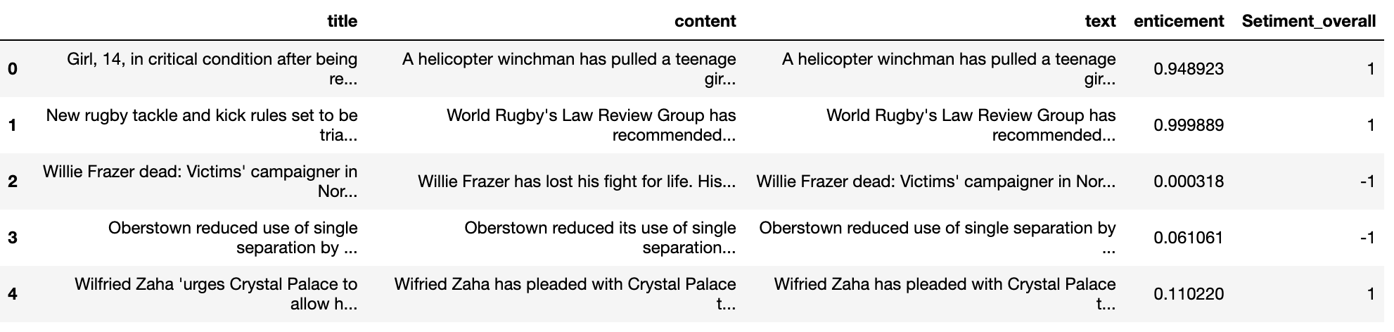
The data contains google news notifications extracted from dataset. The sentimental analysis has been performed on this dataset using EmPushy docker preprocessing image, 1 being postive and -1 being negative sentiments. Let’s import the dataset and see few rows of data.
data = pd.read_csv('google_news_dataset_up.csv')
data.head()
Preprocessing of text field
As we are crating word cloud, we nee to preprocess the text field by removing stopwords, numbers, duplicates and words with character length less than 2. To do so we make use of nltk library stopwords and punctuation.
data_positive = data[data['Setiment_overall']==1]
data_negative = data[data['Setiment_overall']==-1]
Function for cleaning data
def clean_data(data):
    top_N = 100
    #convert list of list into text
    #a=''.join(str(r) for v in df_usa['title'] for r in v)

    a = data['title'].str.lower().str.cat(sep=' ')

    # removes punctuation,numbers and returns list of words
    b = re.sub('[^A-Za-z]+', ' ', a)

    #remove all the stopwords from the text
    stop_words = list(get_stop_words('en'))
    nltk_words = list(stopwords.words('english'))
    stop_words.extend(nltk_words)

    word_tokens = word_tokenize(b)
    filtered_sentence = [w for w in word_tokens if not w in stop_words]
    filtered_sentence = []
    for w in word_tokens:
        if w not in stop_words:
            filtered_sentence.append(w)

    # Remove characters which have length less than 2
    without_single_chr = [word for word in filtered_sentence if len(word) > 2]

    # Remove numbers
    cleaned_data_title = [word for word in without_single_chr if not word.isnumeric()]

    return cleaned_data_title
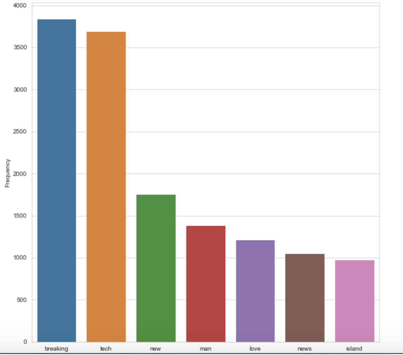
Top frequent words in positive sentences
cleaned_data_title_pos = clean_data(data_positive)
# Calculate frequency distribution
word_dist = nltk.FreqDist(cleaned_data_title_pos)
rslt = pd.DataFrame(word_dist.most_common(top_N),
                    columns=['Word', 'Frequency'])

plt.figure(figsize=(10,10))
sns.set_style("whitegrid")
ax = sns.barplot(x="Word",y="Frequency", data=rslt.head(7))
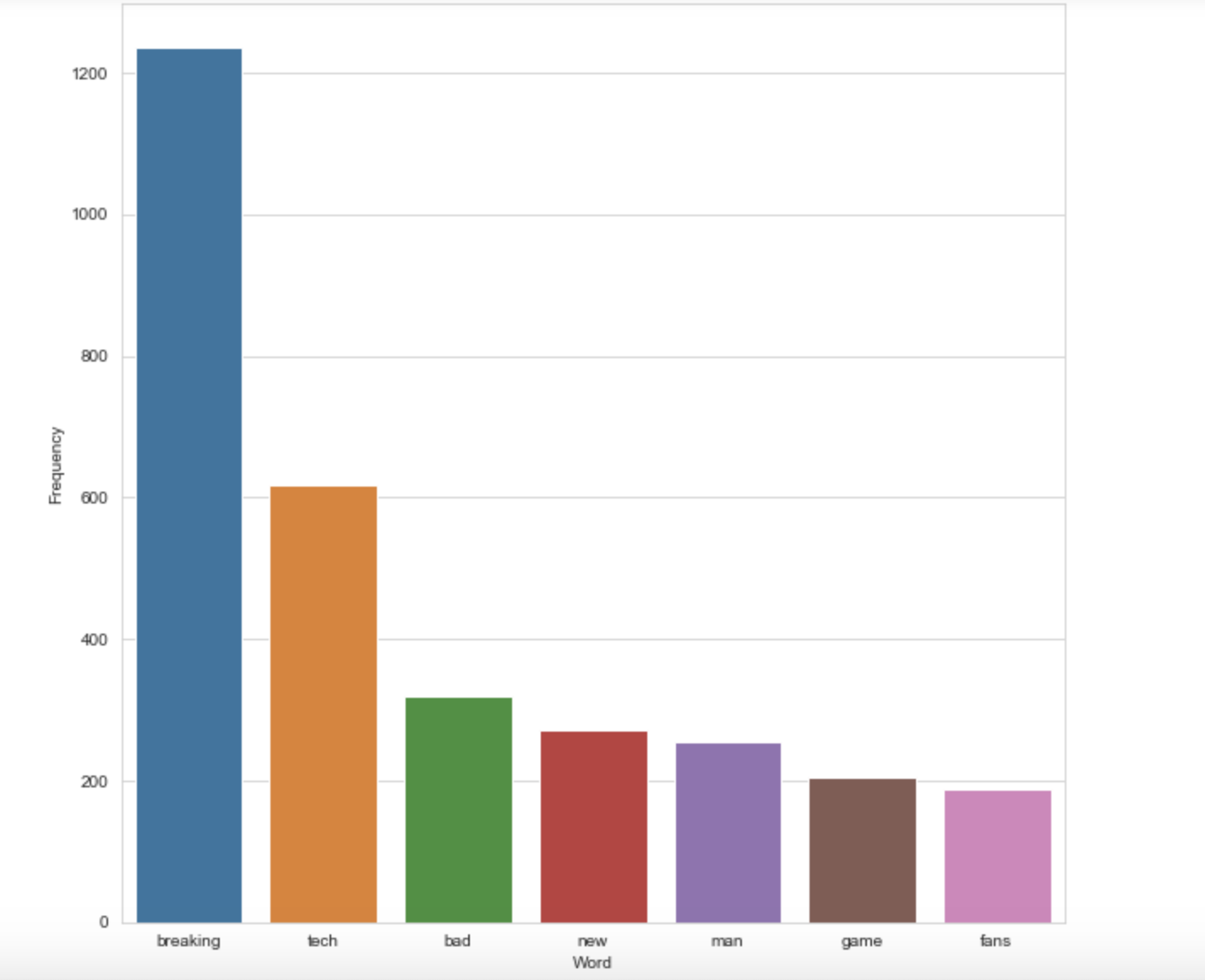
Top frequent words negative sentences
cleaned_data_title_neg = clean_data(data_negative)
# Calculate frequency distribution
word_dist = nltk.FreqDist(cleaned_data_title_neg)
rslt = pd.DataFrame(word_dist.most_common(top_N),
                    columns=['Word', 'Frequency'])

plt.figure(figsize=(10,10))
sns.set_style("whitegrid")
ax = sns.barplot(x="Word",y="Frequency", data=rslt.head(7))
Wordcloud
Define a function to create a wordcloud using WordCloud library.
def wc(data,bgcolor,title, mask):
    plt.figure(figsize = (50,50))
    wc = WordCloud(width = 3000, height = 2000,background_color = bgcolor, max_words = 500,  max_font_size = 100,
                   colormap='rainbow',stopwords=STOPWORDS,mask=mask)
    wc.generate(' '.join(data))
    plt.imshow(wc)
    plt.axis('off')
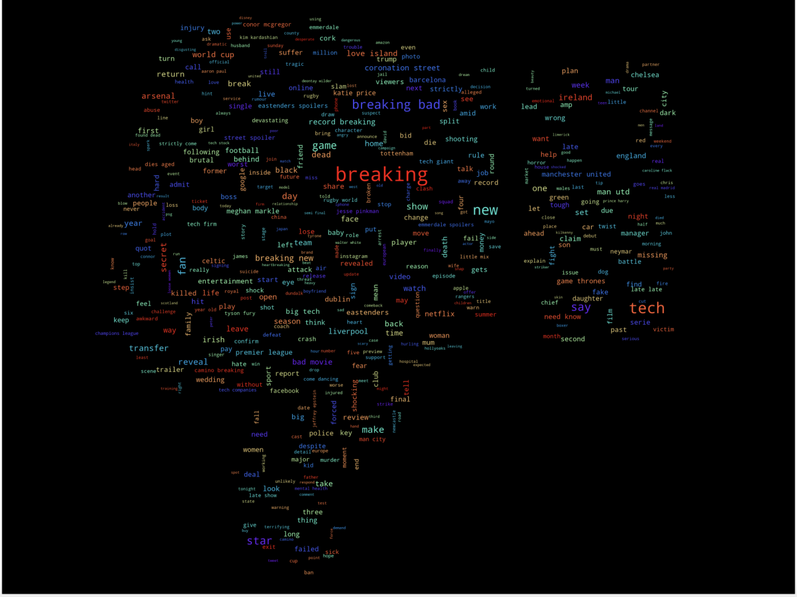
Word cloud without mask
wc(cleaned_data_title_pos,'black','Frequent Words',mask=None )
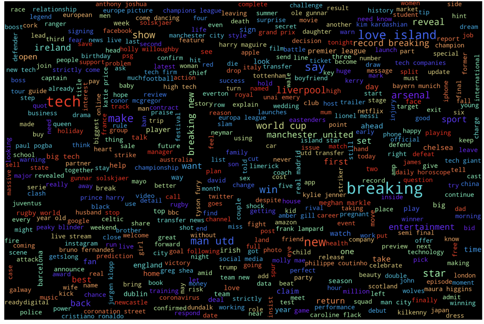
wc(cleaned_data_title_neg,'black','Frequent Words',mask=None )
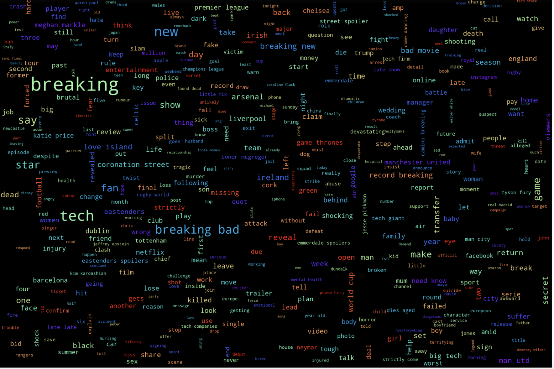
Word cloud with mask
Masks are the shapes used to create a word cloud. Mask should be white background and anyone can download from google. Here I have downloaded thumbsup and thumbs down mask to show positive and negative words used in the text.
img = Image.open('upvote_up.png')
img.resize((20, 20), Image.ANTIALIAS)
plt.imshow(img)
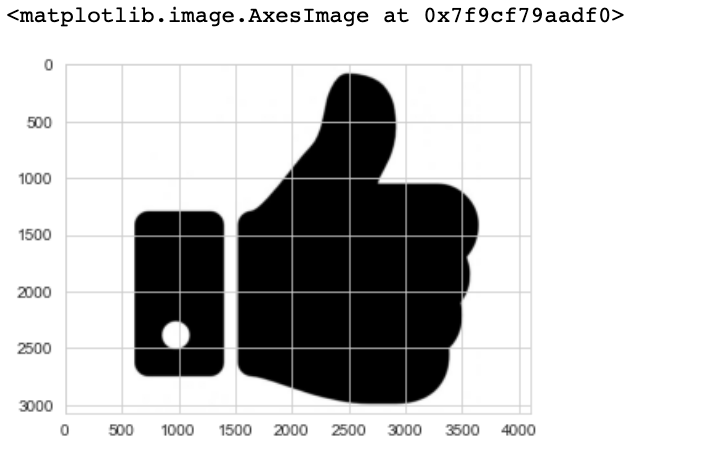
img = Image.open('downvote_up.png')
img.resize((20, 20), Image.ANTIALIAS)
plt.imshow(img)
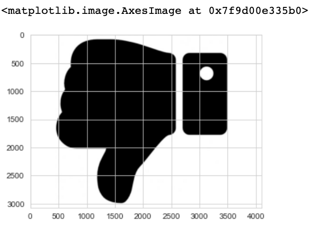
Now call the function wc created before and send mask as an argument as I have already created function to facilitate the mask.
Positive sentiment using thumbs up mask
Load the thumbsup mask and call the function to create the wordcloud by passing mask as an argument.
mask_pos = np.array(Image.open('upvote_up.png'))
wc(cleaned_data_title_pos,'black','Common Words', mask_pos)
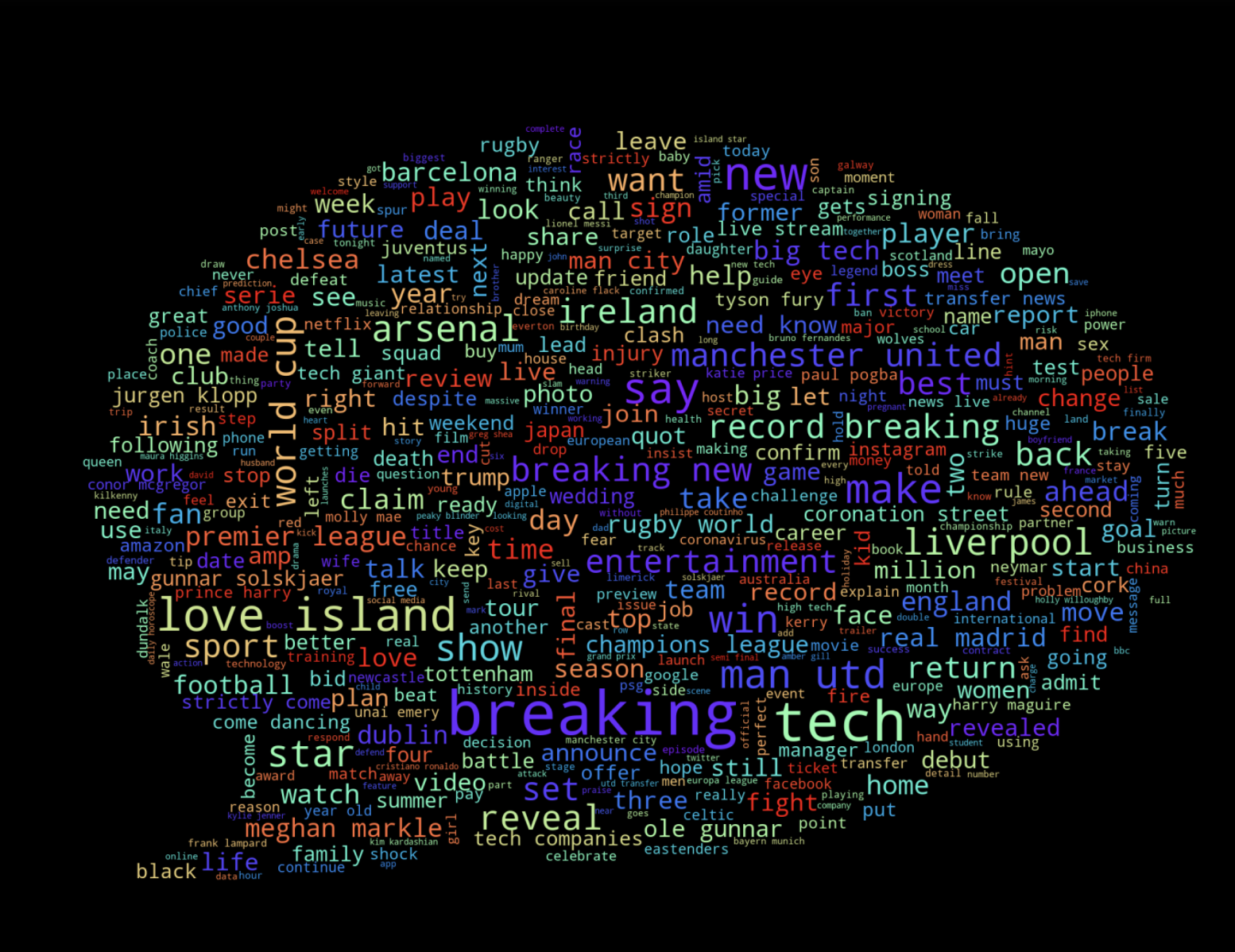
Negative sentiment using thumbs down mask
Load the thumbsdown mask and call the function to create the wordcloud by passing mask as an argument.
mask_neg = np.array(Image.open('downvote_up.png'))
wc(cleaned_data_title_neg,'black','Common Words', mask_neg)
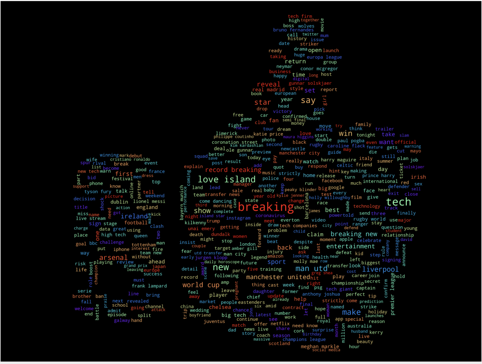
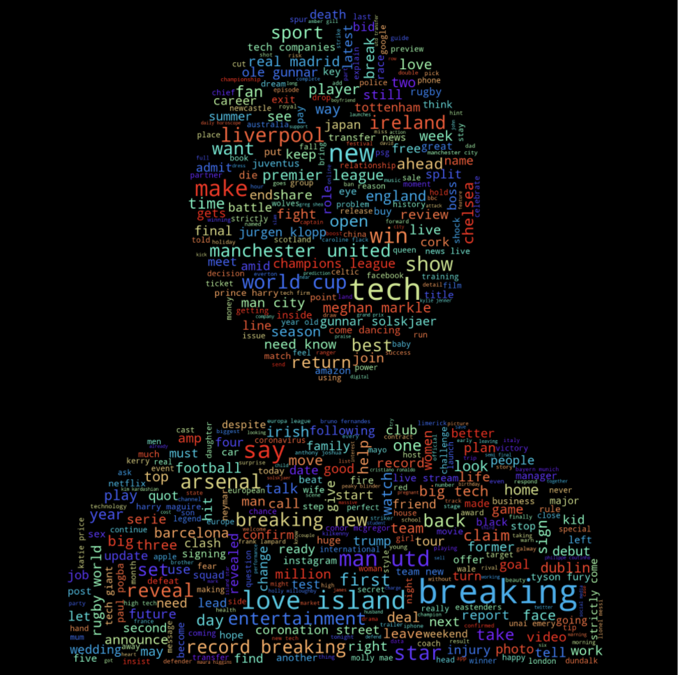
Comment mask to show most words used in comments
mask_com = np.array(Image.open('comment.png'))
wc(cleaned_data_title_pos,'black','Common Words', mask_com)
Star mask to show common words in the comments selected as Editor`s pick
mask_star = np.array(Image.open('star.png'))
wc(cleaned_data_title_pos,'black','Common Words', mask_star)

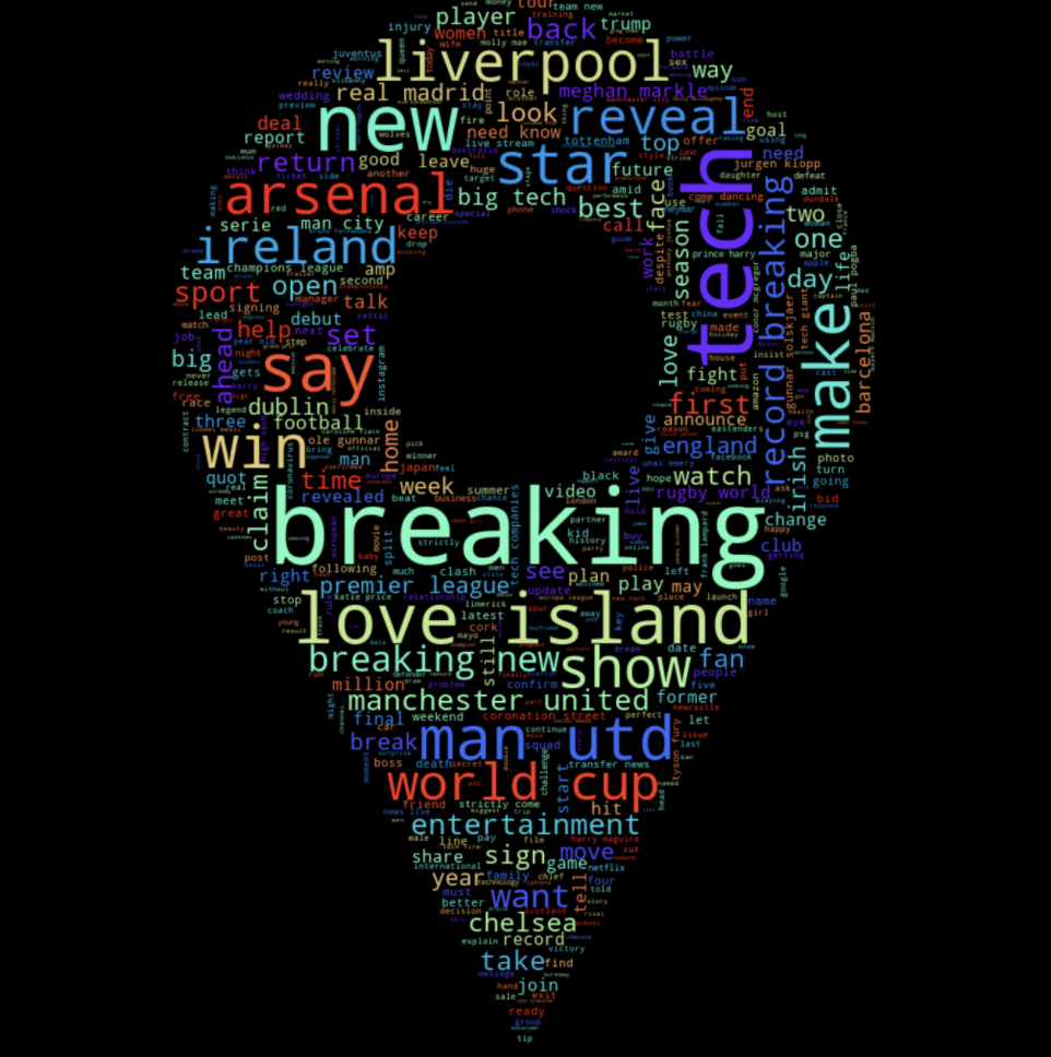
Location mask to show most common locations of the commenters
In this dataset I do not have location, so Iam using few words only to create it.
mask_loc = np.array(Image.open('loc.png'))
wc(cleaned_data_title_pos,'black','Common Words', mask_loc)
User mask to show Usernames with most comments
mask_user = np.array(Image.open('user.png'))
wc(cleaned_data_title_pos,'black','Common Words', mask_user)
Function to save the image
def wc(data,bgcolor,title, mask):
    plt.figure(figsize = (50,50))
    wc = WordCloud(width = 3000, height = 2000,background_color = bgcolor, max_words = 500,  max_font_size = 100,
                   colormap='rainbow',stopwords=STOPWORDS,mask=mask)
    wc.generate(' '.join(data))
    plt.imshow(wc)
    plt.axis('off')
    plt.savefig('data_ps_white.jpg')
### Conclusion As demonstrated we can create word clouds of any shape using masks which are great and effective of visualisation.
### References